Spatial Transformer Network

Spatial Transformer Network(STN)

Introduction

---

CNN is not invariant for scaling and rotaion.

---

STN核心由localization网络、网络生成器、网络采样器组成：

localization一般有卷积层和全连接层组成，用以学习仿射变换参数$\theta$；

网络生成器根据学习到的$/theta$建立从输出到输入的坐标映射网络$T_{\theta}$；

网络采样器通过插值的方法计算输出图像每个像素的像素值。

---

STN的突出优点是不需要矫正的标签进行训练，而是自适应学习最优的空间变换，以便于网络的后续部分更好的处理数据。

Code based digit recognition

from __future__ import print_function  # 即使在python2.X，使用print就得像python3.X那样加括号使用
import torch
import torch.nn as nn
import torch.nn.functional as F
import torch.optim as optim
import torchvision
from torchvision import datasets, transforms
import matplotlib.pyplot as plt
import numpy as np

#加载数据
device = torch.device("cuda" if torch.cuda.is_available() else "cpu")
# Training dataset
train_loader = torch.utils.data.DataLoader(
    datasets.MNIST(root='.', train=True, download=True,
                   transform=transforms.Compose([
                       transforms.ToTensor(),
                       transforms.Normalize((0.1307,), (0.3081,))
                   ])), batch_size=64, shuffle=True, num_workers=4)
# Test dataset
test_loader = torch.utils.data.DataLoader(
    datasets.MNIST(root='.', train=False, transform=transforms.Compose([
        transforms.ToTensor(),
        transforms.Normalize((0.1307,), (0.3081,))
    ])), batch_size=64, shuffle=True, num_workers=4)

#建立手写数字识别模型
class Net(nn.Module):
    def __init__(self):
        super(Net, self).__init__()
        self.conv1 = nn.Conv2d(1, 10, kernel_size=5)  # in_channel, out_channel, kennel_size
        self.conv2 = nn.Conv2d(10, 20, kernel_size=5)
        self.conv2_drop = nn.Dropout2d()
        self.fc1 = nn.Linear(320, 50)
        self.fc2 = nn.Linear(50, 10)

        # Spatial transformer localization-network
        # 其实这里的localization-network也只是一个普通的CNN+全连接层
        # nn.Conv2d前几个参数为in_channel, out_channel, kennel_size, stride=1, padding=0
        # nn.MaxPool2d前几个参数为kernel_size, stride=None, padding=0, dilation=1, return_indices=False, ceil_mode=False
        self.localization = nn.Sequential(
            nn.Conv2d(in_channels=1, out_channels=8, kernel_size=7),
            nn.MaxPool2d(2, stride=2),
            nn.ReLU(True),
            nn.Conv2d(8, 10, kernel_size=5),
            nn.MaxPool2d(2, stride=2),
            nn.ReLU(True)
        )

        # Regressor for the 3 * 2 affine matrix
        self.fc_loc = nn.Sequential(
            nn.Linear(10 * 3 * 3, 32),  # in_features, out_features, bias = True
            nn.ReLU(True),
            nn.Linear(32, 3 * 2)
        )

        # Initialize the weights/bias with identity transformation
        self.fc_loc[2].weight.data.zero_()
        self.fc_loc[2].bias.data.copy_(torch.tensor([1, 0, 0, 0, 1, 0], dtype=torch.float))

    # Spatial transformer network forward function
    def stn(self, x):
        xs = self.localization(x)  # 先进入localization层
        xs = xs.view(-1, 10 * 3 * 3)  # 展开为向量
        theta = self.fc_loc(xs)  # 进入全连接层，得到theta向量
        theta = theta.view(-1, 2, 3)  # 对theta向量进行resize操作，输出2*3的仿射变换矩阵,通道数为C

        # affine_grid函数的输入中，theta的格式为(N,2,3)，size参数的格式为(N,C,W',H')
        # affine_grid函数中得到的输出grid的大小为(N,H,W,2)，这里的2是因为一个点的坐标需要x和y两个数来描述
        grid = F.affine_grid(theta=theta, size=x.size())  # 这里size参数为输出图像的大小，和输入一样，因此采取x.size
        # grid_sample函数的输入中，x代表ST的输入图，格式为(N,C,W,H),W'可以不等于W,H‘可以不等于H;grid是上一步得到的
        x = F.grid_sample(x, grid)

        return x

    def forward(self, x):
        # transform the input
        x = self.stn(x)

        # Perform the usual forward pass
        x = F.relu(F.max_pool2d(self.conv1(x), 2))
        x = F.relu(F.max_pool2d(self.conv2_drop(self.conv2(x)), 2))
        x = x.view(-1, 320)
        x = F.relu(self.fc1(x))
        x = F.dropout(x, training=self.training)
        x = self.fc2(x)
        return F.log_softmax(x, dim=1)


model = Net().to(device)

# 训练模型
optimizer = optim.SGD(model.parameters(), lr=0.01)


def train(epoch):
    model.train()
    for batch_idx, (data, target) in enumerate(train_loader):
        data, target = data.to(device), target.to(device)

        optimizer.zero_grad()
        output = model(data)
        loss = F.nll_loss(output, target)  # 前面用的是log_softmax，因此这里用nll_loss
        loss.backward()
        optimizer.step()
        if batch_idx % 500 == 0:
            print('Train Epoch: {} [{}/{} ({:.0f}%)]\tLoss: {:.6f}'.format(
                epoch, batch_idx * len(data), len(train_loader.dataset),
                100. * batch_idx / len(train_loader), loss.item()))

def test():
    with torch.no_grad():
        model.eval()
        test_loss = 0
        correct = 0
        for data, target in test_loader:
            data, target = data.to(device), target.to(device)
            output = model(data)

            # sum up batch loss
            test_loss += F.nll_loss(output, target, reduction='sum').item()
            # get the index of the max log-probability
            pred = output.max(1, keepdim=True)[1]
            correct += pred.eq(target.view_as(pred)).sum().item()

        test_loss /= len(test_loader.dataset)
        print('\nTest set: Average loss: {:.4f}, Accuracy: {}/{} ({:.0f}%)\n'
              .format(test_loss, correct, len(test_loader.dataset),
                      100. * correct / len(test_loader.dataset)))

#可视化数据
def convert_image_np(inp):
    """Convert a Tensor to numpy image."""
    inp = inp.numpy().transpose((1, 2, 0))
    mean = np.array([0.485, 0.456, 0.406])
    std = np.array([0.229, 0.224, 0.225])
    inp = std * inp + mean #逆正则化
    inp = np.clip(inp, 0, 1)
    return inp

# We want to visualize the output of the spatial transformers layer
# after the training, we visualize a batch of input images and
# the corresponding transformed batch using STN.


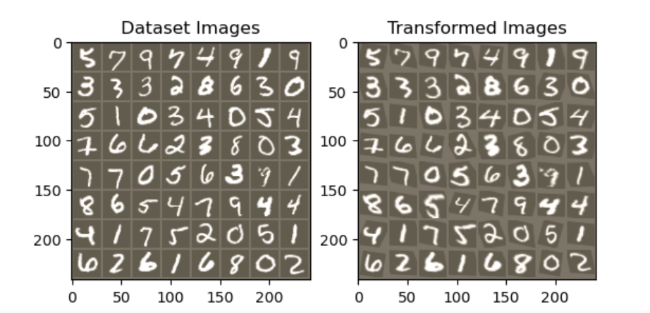
def visualize_stn():
    with torch.no_grad():
        # Get a batch of training data
        data = next(iter(test_loader))[0].to(device)

        input_tensor = data.cpu()
        transformed_input_tensor = model.stn(data).cpu()

        in_grid = convert_image_np(
            torchvision.utils.make_grid(input_tensor))

        out_grid = convert_image_np(
            torchvision.utils.make_grid(transformed_input_tensor))

        # Plot the results side-by-side
        f, axarr = plt.subplots(1, 2)
        axarr[0].imshow(in_grid)
        axarr[0].set_title('Dataset Images')

        axarr[1].imshow(out_grid)
        axarr[1].set_title('Transformed Images')

if __name__ == '__main__':
    for epoch in range(1, 20 + 1):
        train(epoch)
        test()

    # Visualize the STN transformation on some input batch
    visualize_stn()

    plt.ioff()
    plt.show()

下图展示了STN处理后的图像变化结果：